Ohio economists: extending child work hours will not develop tomorrow's workforce

In a survey released this morning by Scioto Analysis, the majority of economists surveyed thought the proposed extension of hours eligible to be worked by 14 and 15 year olds would not meaningfully help these teenagers develop human capital. Senate Bill 30 would allow these teenagers to work until 9:00 p.m. during the school year, currently they can only work as late as 7:00 p.m. most nights.

Kevin Egan of the University of Toledo writes “the overall limit for hours worked for this group is the same, it just allows later hours to 9 pm. I expect very small to no impact on learning and human capital development, as the only change is allowing the hours of work to be a little later.”

Additionally, the majority of economists surveyed think this proposal might decrease safety for young workers. Jonathan Andreas of Bluffton University, one economist who agrees wrote “... not a big change, but it would increase the number of days that kids are commuting home after dark and the number of hours working after dark and more accidents happen after dark.”

The economists who disagreed pointed to the fact that some teenagers might substitute other risky behavior for later working hours. “14 and 15 year olds are probably safer with employers than other ways they would spend their time,” writes David Brasington of the University of Cincinnati. 

The Ohio Economic Experts Panel is a panel of over 40 Ohio Economists from over 30 Ohio higher educational institutions conducted by Scioto Analysis. The goal of the Ohio Economic Experts Panel is to promote better policy outcomes by providing policymakers, policy influencers, and the public with the informed opinions of Ohio’s leading economists.

Should hybrid cars pay for roads?

The Ohio House of Representatives recently passed a two-year, $12.6 billion transportation budget.

The budget included a number of different provisions, including billions of dollars for pavement and bridges, dollars allocated specifically for economic development projects, and $3 billion for Cincinnati’s Brent Spence Bridge.

One small provision of the bill, however, makes a tweak to the current hybrid car registration process. This change will reduce the registration fee for a plug-in hybrid vehicle from $200 to $100 on Jan. 1, 2024.

Fees for hybrid and electric vehicles have been a bit of a political football over the past few years of Ohio politics. Fiscal conservatives have increased fees hoping to recoup some of the losses to the state from reduced gas tax fees. Environmentalists have decried this policy, saying public policy should be rewarding use of electric and hybrid cars, not discouraging it.

In 2019, Scioto Analysis released a white paper that is pertinent to this conversation. In this paper, we highlight the four major costs of vehicles on the road.

First, there is congestion. The more vehicles on the road, the harder it is to drive and the more time people spend in vehicles driving than at their destination. This exacts a cost on society in the form of time.

Second, there are crashes. More vehicles on the road means more people dying from motor vehicle crashes. This exacts a cost on society in the form of vehicle repair and replacement as well as medical spending and loss of life.

Third, there are emissions. Internal combustion engines emit local emissions that have impacts on local public health and ecosystem health. They also emit carbon, which acts as a greenhouse gas and drives global climate change. These exact costs on society in the form of medical spending, loss of life, and the many dynamic impacts of climate change.

Lastly, more vehicles on the road means more wear and tear on the roads. Since roads are paid for through public spending and are treated as more or less a public good, more vehicles means more costs for taxpayers. This exacts costs on society in the form of more spending on public infrastructure.

Electrification of vehicles (in conjunction with evolution of our energy generation system) can lead to lower emissions. But moving to an electric vehicle will do little for congestion, safety, and infrastructure sustainability.

Gas fees have historically been used as a proxy for infrastructure use. If you drive more, you wear the roads down more. You also buy more gas, which has fees that pay for roads.

The problem the diversification of car fuels presents to this old system of road funding is that now the burden of paying for roads is shifting toward people who have internal combustion engines. This poses concerns for both equity (considering mostly wealthy people own electric cars now) and efficiency (considering those people can now free ride on payments being made by others).

A true 21st-century transportation plan will find a way to implement a vehicle miles traveled fee on all vehicles separate from a gas tax that would capture the cost of emissions. Gas-powered transportation should be more expensive than electric-powered transportation (assuming clean electric generation, which is not really the case today) because of the negative externalities associated with burning of fossil fuels.

Proceeds from fees can be used for rebates for poor drivers or low-income people more broadly, targeted economic development in low-income neighborhoods, or early childhood programs to offset their regressive nature.

We can do transportation policy better in Ohio. And soon enough, we will have to.

This commentary first appeared in the Ohio Capital Journal.

Should we use different discount rates for different projects?

The discount rate is one of the most important considerations of a cost-benefit analysis. It is a critical component that allows us to determine the value we place now on benefits that do not accrue until later. 

Essentially, the discount rate is how we measure uncertainty about the future value of our expected benefits. For example, $100 of benefits today is better than $100 worth of benefits in 50 years because the world in 50 years will likely be very different from the world today. Therefore, the benefits we earn (or costs we incur) tomorrow might not mean as much as benefits earned today.

In order to determine a policy that has benefits 50 years into the future is more efficient than one that has benefits today, we’d need to factor this uncertainty about future benefits into our cost-benefit analysis.

In policy analysis, the selection of the discount rate can dramatically change how we value different proposals. Higher discount rates mean we are less certain about future benefits, and therefore would prefer projects with short-term gains. If the discount rate is too high, we might be short sighted and not plan far enough ahead as a society, valuing present benefits inordinately over those accrued in the future.

Smaller discount rates often make it more likely that future benefits outweigh short term costs. From a policy perspective, this would lead to much more spending on big investment projects. However, if we don’t discount enough, we might be worse off in the short term for projects that might not pan out very well.

In the United States, the base discount rate recommended by Circular A-4 is 7%. The best practice in cost-benefit analysis is to see if your results are sensitive to changes in the discount rate, but for all projects that is the base number to use. For the vast majority of agencies in the cost-benefit analysis world, a single discount rate across projects is preferred.

However, there is one prominent exception to this rule. Analysts in France use variable discount rates depending on the riskiness of the project. For example, imagine we had to choose between investing in a new hospital or in new railroad infrastructure.

Both have massive short term costs and only begin creating benefits after their completion. The main difference is the riskiness of those benefits actually coming to fruition. The hospital will almost always be a useful investment. The “worst case” scenario for the hospital would be if in the future there were no major disasters or pandemics and those hospital beds remained empty. 

Conversely, the railroad infrastructure is much more likely to not realize its benefits. More railroads are important during strong economic times when there are lots of goods that need to be shipped around, but there are always periods of economic downturn. It is much more likely that we will eventually face a difficult time in the economy than we will suddenly not need hospital beds.

Given the intuitive understanding that the discount rate is a tool we have to measure the risk associated with long term benefits, this approach makes a lot of sense. If we can get an idea of how much risk is associated with each type of policy proposal then we would do a better job of efficiently allocating resources. We can do this by allowing for different discount rates between projects. 

There is little consensus among economists about how to choose discount rates for different policies. Because the discount rate can have a significant impact on the results of cost-benefit analysis, it is important that there is a well defined method in place. Allowing analysts to choose discount rates without any framework to back up their choice could lead to severely biased results, and would open the door to potential manipulation.

Currently, the French government adjusts discount rates by looking at price and income elasticities for the goods generated by a policy proposal. This seems to have some strong promise, but in order to fully understand it, more policy analysis needs to be done using it.

Is early childhood education good economic policy?

Last week I attended the Society for Benefit-Cost Analysis’s annual conference in D.C. This was the first time the Society had met in person in four years, having canceled the 2020 conference just weeks before it was scheduled in March of that year.

This year’s conference was a doozy. Presentations ranged on topics from distilling a large evidence base for a topic to factoring the marginal value of money into cost-benefit analysis to variable discount rates due to risk. But the keynote everyone was excited about was given by Nobel Prize-Winning Economist James Heckman.

James Heckman is 78 years old but speaks with the spryness of someone decades younger. Heckman won the prestigious John Bates Clark Medal in 1983 for his work on time series analysis. In 2000, Heckman was awarded the Nobel Prize in Economics for his work overcoming statistical sample-selection problems.

What makes Heckman so compelling for me, though, is the practicality of his insights. Despite much of Heckman’s work seeming to be rooted in esoteric econometric matters, he has become most famous in policy circles for his championing of early childhood education.

In particular, Heckman has analyzed the long-term effects of two famous early childhood programs: the Perry Preschool Project and the Abecedarian Project. 

The Perry Preschool Project was a randomized early childhood program conducted in the 1960s that we now have six decades of data on. The program was offered to low-income African-American children age three and four who were assessed to be at high risk of school failure. Participants in this early childhood program were arrested less before age 40, had higher income, were more likely to graduate from high school, and even had higher IQs later on.

The Abecedarian Project was a similar program conducted in the 1970s in North Carolina. This study was also a randomized controlled trial but took the treatment a step further, offering education to children starting as infants. Participants ended up with better educational outcomes, higher college matriculation, less teen pregnancy, less marijuana abuse, and less depressive symptoms.

Heckman has championed the Perry Preschool model as not just a model for increasing educational, crime, and earnings outcomes for participants, but even for their children. Now that generational data is available on this program that is over half a century old, Heckman argues that early childhood education is a powerful tool for breaking the cycle of intergenerational poverty.

This research is backed up by the research of another giant of the economic policy world and benefit-cost analysis Timothy Bartik. Bartik started doing applied economic analysis focusing on tax incentives and evaluating how their design contributes to improvements in local wages. He was approached by a foundation that was interested in applying his economic development model to early childhood programs.

The worry these funders had was that local leaders would shy away from funding early childhood programs because the children who receive the education would move away and the benefits would not accrue locally. If this were the case, local policymakers would be funding a program that would be building the workforce of other cities.

Bartik’s research found that indeed these benefits would accrue locally. He used results from the Perry Preschool and Abecedarian projects and found that local wage benefits would outweigh the cost of the programs, even factoring in how many children would move away from the local jurisdiction over their lifetime.

Perry Preschool and the Abecedarian Project are only two small-sample studies, but it is not often that we get a randomized controlled trial with accompanying panel data that follows the participants for decades. Only a handful of studies follow a panel of people through their life course like this one and very few are focused on the results of a randomized controlled trial. While there is always more data to collect and evaluation to conduct, the evidence brought forth by economists like Heckman and Bartik suggest early childhood education is indeed a good investment.

A look at the Ohio Opportunity Index

Recently, the Ohio State University released their Ohio Opportunity Index, a report that measures outcomes for residents across the state at the census tract level. Additionally, they released an interactive dashboard that helps visualize the data. 

Here, I take a look at some of the top findings from the dashboard in Franklin county. Which census tracts are doing well, and where can policymakers find ways to improve peoples’ wellbeing. 

Overall Opportunity

In Franklin county, the area with the lowest overall opportunity score was downtown Columbus. Low opportunity extends North of downtown into the South Linden neighborhood. The German Village neighborhood differs from its neighbors by having a relatively high opportunity score relative to the state as a whole. 

Surrounding suburbs like Bexley and Grandview Heights have very high overall opportunity scores. The farther out suburbs also generally have higher overall opportunity when compared to downtown Columbus, though there are some notable exceptions, especially East of downtown.

Education Opportunity

In Franklin county, the general rule of thumb is that the closer to downtown you get the worse the education opportunity is. Poor education opportunities extend in the North in the neighborhoods between I-70 and I-270. To the west, areas of low opportunity are bounded by I-270. 

One major exception to this rule is Bexley, which sits as an island of high education opportunity near downtown Columbus. The surrounding suburbs also once again areas of much higher educational opportunity when compared to downtown.

Employment Opportunity

One major bright spot for Franklin county is how it scores on employment opportunity. Almost the entire county except for a few census tracts near downtown are near the rank near the top of the state. 

Generally speaking, employment opportunity in the state is higher near the major cities. The more rural parts of Ohio often have lower employment opportunity. In particular, the Appalachian region in the Southwestern part of the state scores poorly on this metric. 

Transport Opportunity

For transportation opportunity, we see that most of the city center actually scores better than some of the surrounding suburbs. There is still a noticeable section of low opportunity tucked in the heart of downtown Columbus, but by and large the city has good transportation. 

The suburbs in Franklin county are fairly mixed in their transportation scores. Most of the distant census tracts score poorly, but there are enough good scores mixed in to prevent this from being a discernible trend.

Health Opportunity

Franklin county scores slightly lower on health opportunity than any of the other metrics mentioned above. The main driver behind this is lower scores in the South suburbs. Broadly, we observe the same areas of low opportunity near the city center with the same neighborhood exceptions in German Village and Bexley.

It is not terribly surprising that many of these scores seem to be correlated with one another. Much of this can likely be attributed to local income and poverty rates. Hopefully, the high job opportunity score in the heart of Columbus might mean that some of these other metrics might begin to improve. 

The utility bailout House Bill 6 made both Ohio’s air and politics dirty

With all the drama surrounding the Householder trial for racketeering, it can be easy to forget the bill behind the former Ohio Speaker of the House’s alleged $60 million payoff from First Energy power company.

House Bill 6 had four major impacts. It required power consumers to bail out two massive nuclear power plants in northern Ohio. It also required Ohio ratepayers to bail out two coal plants: one in Ohio, one in Indiana. It reduced energy efficiency standards, requiring Ohio utilities to reduce energy use by 17.5% rather than the previous goal of 22%. Lastly, it reduced Ohio’s renewable portfolio standard, requiring utilities in Ohio to generate just 8.5% of their power from renewables, lowest in the country among states with standards.

I want to focus on the last impact: reducing Ohio’s renewable portfolio standard.

In 2008, Ohio unanimously passed Senate Bill 221, a bill to require 12.5% of Ohio’s energy to be produced from renewable sources. It was an optimistic time for Ohio’s energy transition.

This optimism started to fray in the 2010s. In 2014, a group of state senators led by now-Congressman Troy Balderson pushed through a bill to freeze the standards in place until 2017. Balderson had originally called for a “permanent freeze” but had it changed to temporary after negotiations with the Kasich administration.

In 2019, Householder pulled off what Balderson couldn’t. With HB 6, he reduced the final goal for Ohio’s renewable energy to 8.5% and pushed back its date from 2022 to 2026.

What will this mean for Ohio? Scioto Analysis released a study in 2021 on carbon emission reductions which found that renewable portfolio standards could be as effective as a carbon tax or a cap-and-trade program at reducing carbon emissions in the state. 

We looked at two approaches: a renewable portfolio of 25% by 2026 based on Michigan’s renewable portfolio standard and a renewable portfolio standard of 80% by 2030 and 100% by 2050 based on Maine’s renewable portfolio standard.

We found that both approaches would be effective at reducing carbon emissions in Ohio and would both drive the global cost of these emissions down from over $45 billion a year to under $25 billion a year.

Reducing reliance on coal and natural gas for power would have ancillary benefits as well. Burning of coal releases contaminants into that air that can lead to respiratory illness. Extraction and production of natural gas can have similar impacts as well as lead to a range of other health impacts.

Use of fossil fuels also poses health equity problems for communities. A 2021 study published in Science Advances found racial-ethnic minorities in the United States are exposed to disproportionately high levels of ambient fine particulate air pollution (PM2.5) than white populations, further compounding inequities already experienced between racial groups. Since Black Ohioans already experience poverty at rates nearly three times as high as white Ohioans, this just compounds inequities in the state.

It’s not often that scandal is so closely wedded to policy, but right now Ohio is dealing with this biggest racketeering charge in history, which stemmed from negotiations over its biggest piece of environmental legislation of the century. Let’s hope we can learn from this and find ways to keep both our air and our politics clean.

This commentary first appeared in the Ohio Capital Journal.

How to be a bayesian policy analyst

By and large, humans are pretty bad at understanding probabilities. We live in a world of tangible things and real events which makes it hard to wrap our heads around the abstract concept of randomness. 

Among statisticians, there are two broad philosophies when it comes to thinking about uncertainty: frequentist statistics and bayesian statistics. 

Frequentist statistics assumes that there is some true probability distribution from which we randomly observe some data. For example, imagine we were flipping a coin and trying to determine if it was fair or not. 

A frequentist would design an experiment, and determine a hypothesis test. “I am going to flip the coin 50 times, and I will say the coin is not fair if I get less than 20 or more than 30 heads.”

From this frequentist experiment, we will be able to produce a p-value and a confidence interval. These tell us about the probability of observing our particular set of 50 coin flips, out of the universe of all possible sets of 50 coin flips.

On the other hand, Bayesian statistics relies on our prior knowledge about random variables as the foundation model. These prior assumptions can be the result of historical data or simply the statisticians' judgment.

Take the same coin flipping experiment, we no longer begin by defining a null hypothesis and some criteria to reject it. Instead, we begin with a prior distribution, perhaps assuming the coin is fair, and our goal is to create a “posterior distribution.” In this case, the posterior would be what is the probability the coin is fair.

Assume now that we ran our experiment and flipped 21 heads in 50 tries. In this case, the frequentist would say “We fail to reject the null hypothesis and can not conclude whether or not the coin is fair.” The Bayesian would instead find the posterior distribution, and be able to make a statement about the probability the coin is fair.

In short, the frequentist will never calculate the probability of a hypothesis being true. They will either reject it or fail to reject it. A Bayesian statistician will always begin with a prior guess about whether a hypothesis is true, and update that prior guess as they observe new information.

I personally find Bayesian thinking to be a much more satisfying way to conceptualize uncertainty. We all carry around some prior knowledge about how random things should play out, and as we observe new information we update those priors.

However, one thing to realize about intentionally thinking like a Bayesian is that it is often slow to incorporate new and dramatically different pieces of information. This can be good when the dramatically different information is an outlier that we don’t want to have completely determine how we think, but our priors can be slow to recognize when things do change dramatically.

In practice, I still mostly use frequentist statistics as part of my analysis. In practice, Bayesian analysis is often sensitive to the construction of the prior distribution and it is not always useful to a policy maker when the result of some analysis still has probability baked in.

Still, Bayesian statistics reminds us that we live in a world where things are uncertain. Especially in policy analysis, where we often try to predict future outcomes, it is important to remember that there is uncertainty and unlikely outcomes do not necessarily mean our predictions were wrong.

Ohio economists pessimistic about proposed school voucher program

In a survey of Ohio economists released this morning by Scioto Analysis, the majority of respondents disagreed or were uncertain that the proposed increase of Ohio’s private school voucher program would increase standardized test scores for Ohio’s students. “There are a lot of complex dynamics (some students may see higher scores but others may see lower scores) but almost certainly there will not be a significant effect on the average test scores in the state,” said Dr. Curtis Reynolds of Kent State. 

When asked if the proposed voucher increase would lower the quality of Ohio’s public schools, 11 economists agreed, four disagreed, and seven were uncertain. Dr. Kay Strong, who strongly agreed, said “the proposed upper threshold of $111,000 earning for a family of four assuming two are children will exacerbate the privilege of high income families at the cost of lower quality education from reduced public spending on traditional public school.” 

Since we surveyed the panel, the Ohio senate has introduced Senate Bill 11 which would create universal school vouchers.

The Ohio Economic Experts Panel is a panel of over 40 Ohio Economists from over 30 Ohio higher educational institutions conducted by Scioto Analysis. The goal of the Ohio Economic Experts Panel is to promote better policy outcomes by providing policymakers, policy influencers, and the public with the informed opinions of Ohio’s leading economists.

How to talk about statistics to non-statisticians

The final required class I took in grad school was called “Statistical Consulting,” and unlike every other course I took I did almost no actual statistics in it. Instead, this course predominantly focused on how to take all of the fancy methods and advanced concepts I had learned over the last two years and communicate the results to people without a background in statistics. 

As a policy analyst, I find myself communicating with non-statisticians more often than in school. This is an exciting opportunity to share the statistical tools I have with an audience that can meaningfully apply my results. These are some of the things I learned that have helped me better explain complicated concepts to a less technical audience.

Ask your audience for their statistical background

During my first ever consulting project as a grad student, I spent about 10 minutes of my first meeting going over the pros and cons of using a time-series approach with the client before they had the opportunity to ask me what a time-series model was. This is not to say that the discussion on the pros and cons of the time series approach was wrong or that the client didn’t need to be included in that conversation, but rather that had I known my client’s background I would have approached that discussion differently.

In this particular case, my client wasn’t interested in the statistical differences between the models I was proposing, but rather what the practical differences would be in the final report. After resetting, we were able to have a much more productive discussion that was tailored to his level of understanding. 

Use visuals when possible

Good data visualizations can communicate a complicated idea almost instantly, especially when paired with a clear written description of the main takeaways. However, it is important to not get carried away with visualizations. 

One common mistake is visualizing every possible part of an analysis. Visuals are great for highlighting the most important parts of a report. Highlighting everything might make it harder to find the most important pieces of information. 

Another consideration to have is when to use a graph or a table to visualize data. A general rule of thumb is to use tables when the specific value of a result is important and graphs when the broader trend is important. 

Provide context

Statistics never exist in a vacuum, and it is important to provide context in order to make your results more useful. Being upfront about what data or methods you used, what the strengths or weaknesses of your approach were, these are the sort of non-result pieces of information that help people understand the full picture of an analysis. 

Be honest

There are a whole lot of approaches we can use when analyzing data, and some of these approaches might allow for different interpretations of the results. Statistics sometimes gets viewed as a scientific and objective way to examine the world around us (which it largely is), but the perspective of the analyst has a lot of weight in determining the final message. 

Always make sure you are being clear about the assumptions your models make, and the limitations of your results. It goes without saying that intentionally misleading charts or excluding critical information has no place in any respectable analysis.

How do Americans spend their free time?

A central theory of labor economics covered in most introductory microeconomics courses is that of the “labor/leisure tradeoff.” This is the concept that workers have time they can spend working and time they can spend doing other things and that they will try to maximize their “utility” by achieving the optimal mix between labor and leisure.

Below is a visualization of the concept. You can plot a wage on a chart like this as a line that runs from the top left to the bottom right and a worker will choose how much to work based on where their wage line intersects the “indifference curve” (the blue lines) that is furthest out. An “indifference curve” represents all the points as which a worker would be “indifferent” to a different mixture between income and leisure. 

So a worker is just as happy at being at point A or point B who has the indifference curve IC1, though at point A she has more income and less leisure and point B she has more leisure and less income. Any point to the northeast of IC1 is preferable to any point on IC1 because it means more income and more leisure, less leisure compensated by much more income, or less income compensated by much more leisure.

This is of course a simplification. There are structural frictions in the labor market that can limit a worker from achieving the appropriate mix of labor and “leisure” that she desires. But empirically we do see this phenomenon playing out, with price increases like taxes leading to reductions in labor time in favor of “leisure” time. What I’m more interested in talking about here is something else: what we define as “leisure.”

“Leisure” time is defined by this model as time a worker spends doing something other than generating income. But is all of this rightly understood as “leisurely” activity?

One place we can look to find an answer to this question is the American Time Use Survey. The American Time Use Survey is a nationally representative survey conducted by the Census Bureau to determine how, where, and with whom Americans spend their time. It is the only federal survey providing data on the full range of non-market activities, from childcare to volunteering.

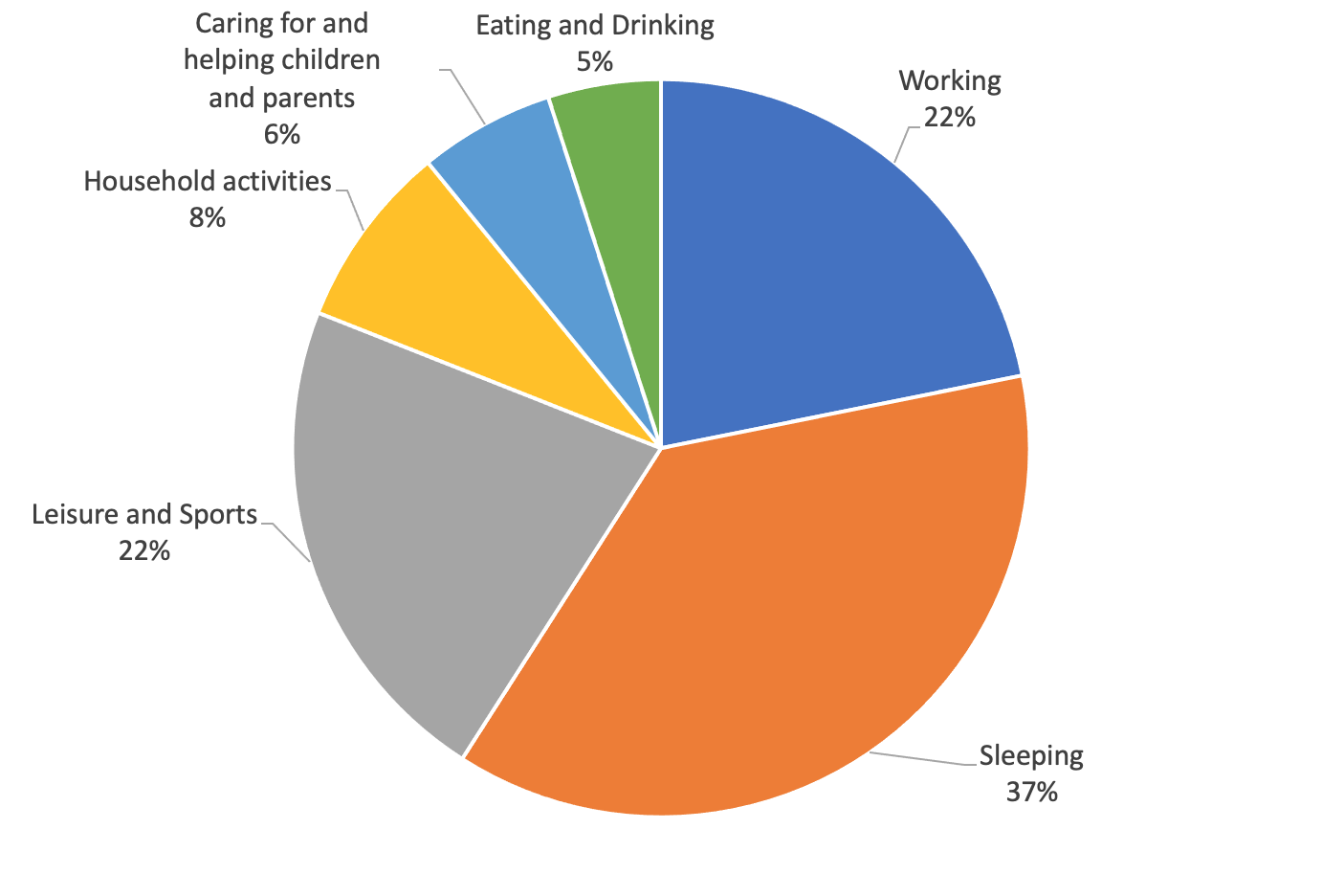
Looking at an overview of how Americans spend their time, the picture of “leisure time” gets a little more complex.

According to 2021 results, Americans spend about 22% of their time on average at work. They spend about 37% of their time on sleeping, 22% of their time on leisure and sports, 8% of their time on household activities (including travel), 6% of their time on care for children and parents, and about 5% of their time on eating and drinking.

So if we look at these results, we find that 42% of total time (54% of what the labor/leisure model calls “leisure time”) is spent on eating and sleeping, activities most people would deem essential to survival. Yes, there is a leisure component to eating and sleeping, but many people’s experience with food and sleep in the United States would not necessarily be called “leisurely.”

Another 14% of total time (18% of “leisure time”) is spent on household activities and caring for family members. This is what many would consider “non-market economic activity”--dollars aren’t changing hands, but they certainly could if these activities were outsourced from the household to a cleaning service, child care agency, or long-term care facility.

This only leaves 22% of total time, or 28% of time not worked, as time for “leisure and sports.” So only about a quarter of what we call “leisure time” is truly spent doing things we consider “leisure.”

When I was in graduate school, our economics professor eschewed the use of the phrase “leisure time” for the phrase “non-market time.” I think this is probably a better way to treat this time we spend sleeping, eating, taking care of family, caring for the house, and on leisure and exercise.